Using Apache Superset to visualize simulation data
How can data that is generated through a mosaik simulation be explored without too much hassle and programming knowledge? In this tutorial we will look at Apache Superset, an open source tool for data exploration and visualization. This tutorial is divided into two parts, the installation of Apache Superset and how to couple it with mosaik and the basic usage of Superset. For a more in-depth look at Apache Superset and all of its features please consult the tutorials on the Superset website.
This tutorial is based on a superset and timescaledb instance. Both instances were run through docker on ubuntu.
Getting Started
In this part of the tutorial we will show you how to install the necessary tools to use Apache Superset with mosaik.
Installing a database and collecting data
To use Apache Superset a SQL database that contains simulation data is needed. For this there are currently three options in mosaik.
To install one of the databases locally follow corresponding the link. (This tutorial is written with the Timescale database in mind. However, the other databases, should follow similar steps.)
Make sure to change the port of the database to something different from 5432 if you want to run the database and superset locally, as superset uses the same default port for its databse. When using docker the command should look something like this:
$ docker run -d --name [YOURCONTAINERNAME] -p [YOURPORT]:5432 ...
After installing the database the corresponding mosaik adapter can be used to save simulation data into the database:
For further explanation regarding this.
Installing Superset
This tutorial is written using the production version of Superset based on the commit 0c083bdc1af4e6a3e17155246a3134cb5cb5887d .
To install the production version of Superset locally clone the Superset repository using the following command:
$ git clone https://github.com/apache/superset.git
$ cd superset
Afterwards a secret key needs to be set for the production version. For this the file superset_config.py is needed. It can be copied into the right place using the command:
$ cp ./docker/pythonpath_dev/superset_config_local.example ./docker/pythonpath_dev/superset_config_docker.py
When this is done a Secret Key can be generated. The following command can be used on linux:
$ openssl rand -base64 42
and then be added into the superset_config ./docker/pythonpath_dev/superset_config_docker.py like so:
$ SECRET_KEY = 'YOUR_OWN_RANDOM_GENERATED_SECRET_KEY'
Please be sure to remove any other option from the configuration or make sure you need the other configuration options and know what they do.
The Superset instance can be started with the following commands:
$ docker-compose -f docker-compose-non-dev.yml pull
$ docker-compose -f docker-compose-non-dev.yml up
Afterwards the instance can be found at the webaddress http://localhost:8088/. The default login username and password are admin.
Connecting Superset with the Mosaik database
To connect superset with the database both superset and the database need to be online.
This connection is done in the superset web application.
The connection between superset and the database is done in the settings -> Database Connections menu.
Database Connections Setting
Afterwards a new Database is added by clickin on the Database + Button.
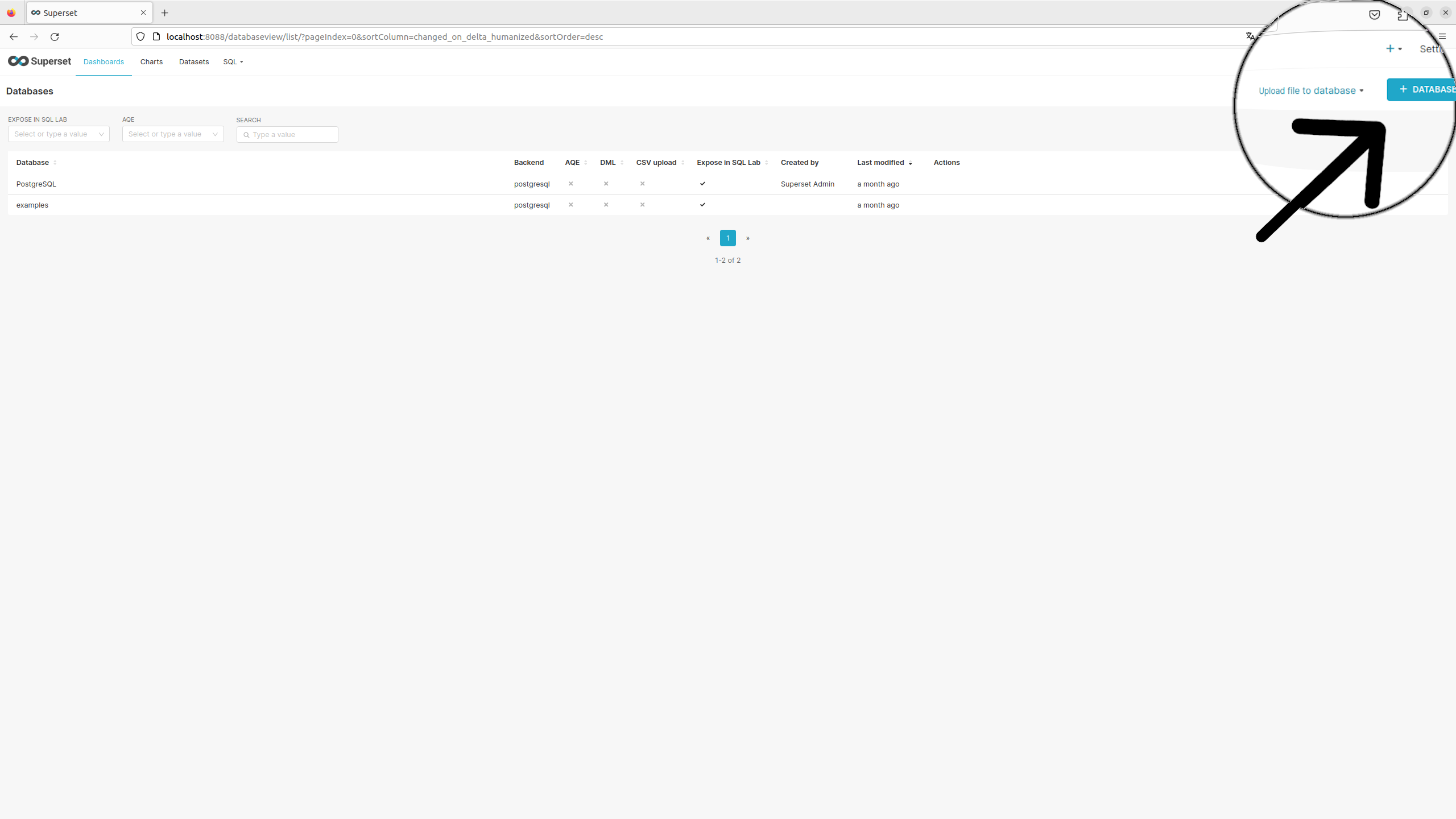
Button to click for adding a database
This initiates the add database dialog consisting of three steps:
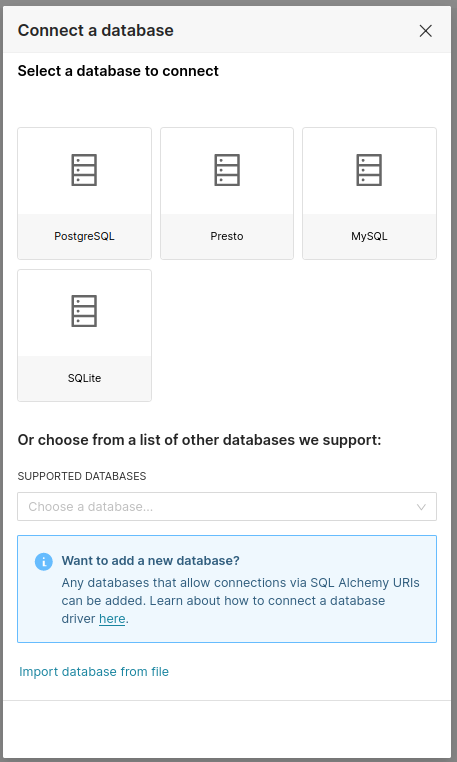
Step 1: Choosing the correct database(PostgreSQL in this example)

Step 2: Adding the database Credentials. If the database i run locally the IP-Address is 172.18.0.1 by default. If using Windows the IP might be host.docker.internal.
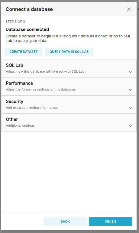
Step 3: Finishing the setup
Visualizing Data in Apache Superset
After connecting the database to superset the data can now be visualized. This tutorial shows data that is saved in a Timescale database. This data is saved using the MultiWriter2 of the mosaik Timescale adapter. To do this first the data needs to be extracted from the databae using SQL. This is done in the SQL Lab:
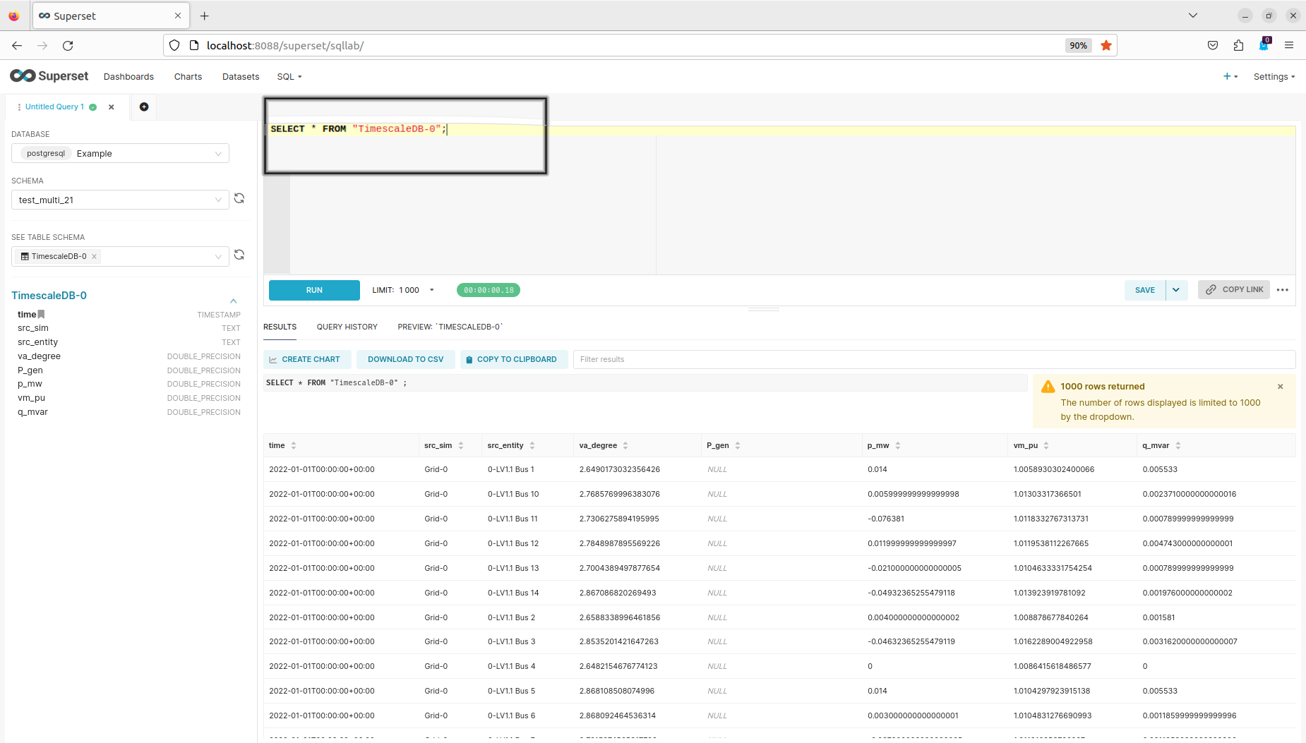
View of the SQL Lab
I the SQL Lab the database the database, schema and table schema of a table in the database can be selected on the left side. On the right side a sql query can be built. In this example we use a simple query to get all of the data from the table. If you are using the single writer from the mosaik timescale component the SQL query will look a bit different with it either being a double cast in case of the json table_type:
SELECT time, CAST(CAST(values->'Grid-0.0-LV1.1 Bus 1' AS VARCHAR) AS DOUBLE PRECISION) AS "BUS 1" FROM testing_json
 WHERE value_type = 'va_degree'
And it being a single cast when it being the table_type string:
SELECT time, CAST(value AS DOUBLE PRECISION) FROM testing_string
 WHERE value_type = 'va_degree'
After extracting the wanted data using a SQL query it needs to be saved as a dataset by running the query and afterwards using the save button:
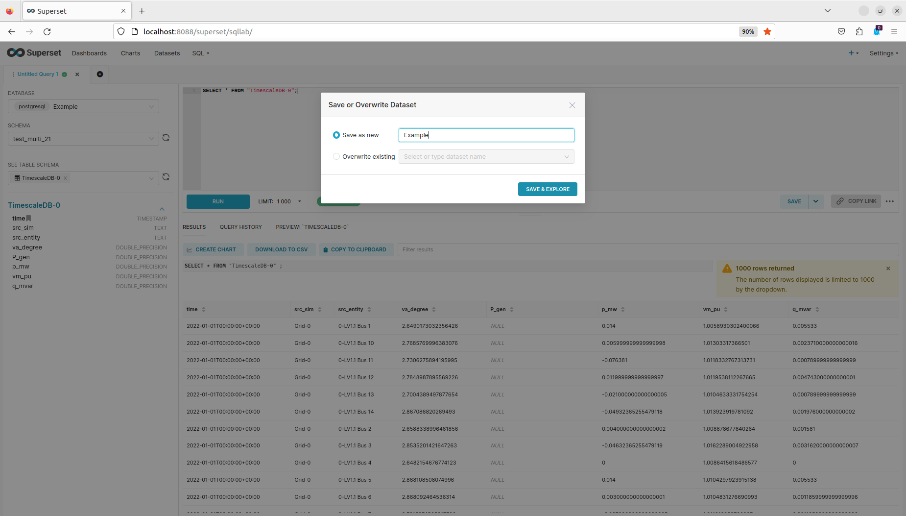
View of saving the dataset in the SQL Lab
Clicking the Save & Explore Button will open up the Chart creation view of superset. This can also be done afterwards by selecting the wanted dataset in the datasets tab.
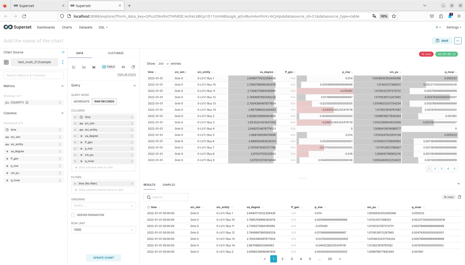
Chart View of superset
The default chart view of superset can be divided into two important parts. The left side where you can chose the kind of chart to create as well as input the data from the dataset into the chart and the right chart where the chart will be displayed.
For this example lets start by selecting a line chart from the left side and then adding data to the relevant fields.
Changing chart to line chart.
After changing the chart to line chart the relevant fields to fill out are the x-Axis, which in most cases will be the time column, and the metrics, which represent te y values. Superset can not display simple y value, it is always a sql function. If a simple x/y comparison is needed the avg/min/max of the y values can be used since for only one value this is the value itself.
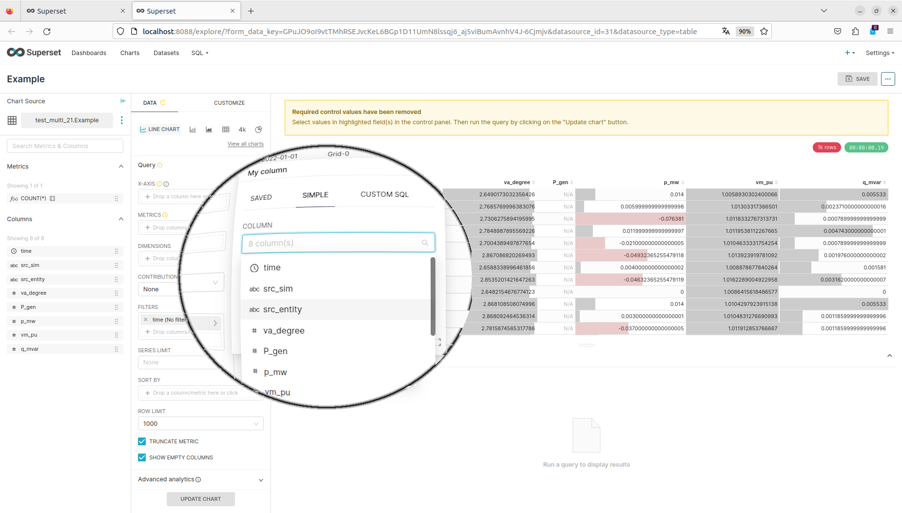
For selecting the x Axis you can chose from your dataset columns. Most of the time you want the simple time value but a custom sql query can also be used.
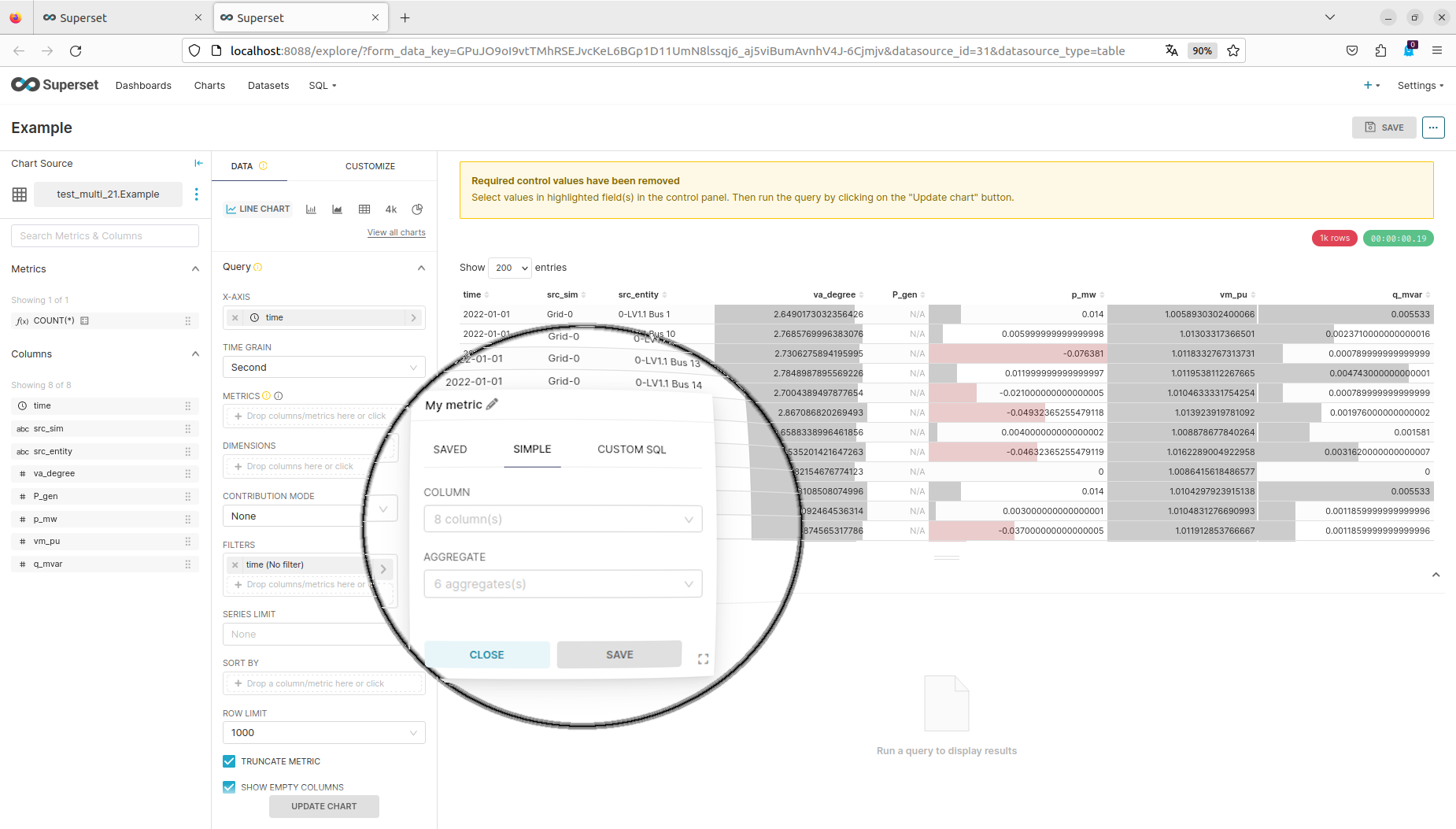
When selecting a metric there are many basic sql aggregation functions to choose from.
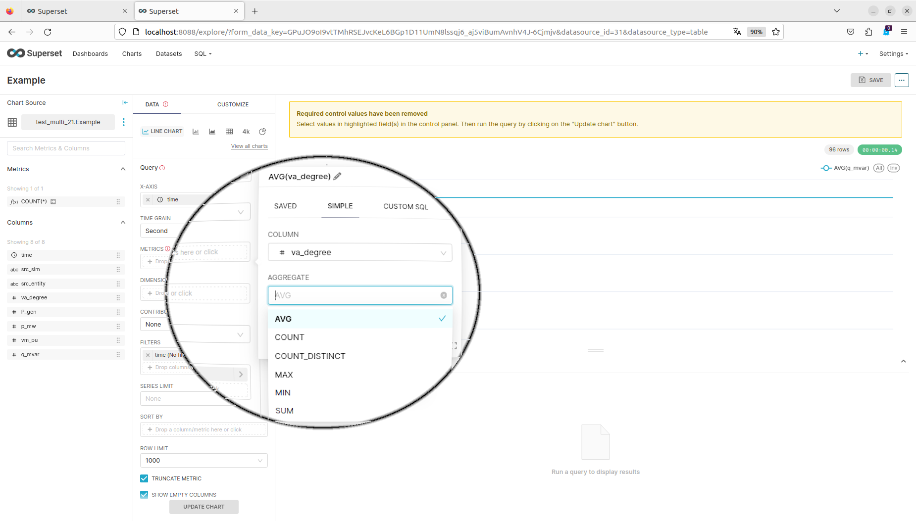
After selecting the metrics you can render the chart by clickin the Create Chart or Update Chart button
Multiple metrics can be selected but only one x-Axis.
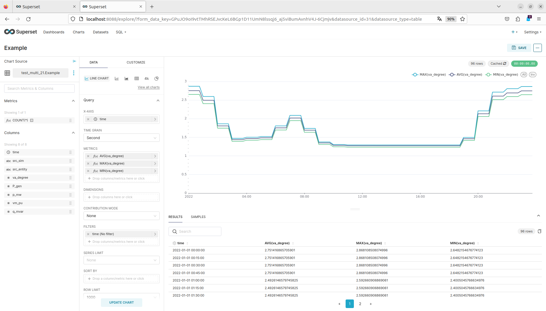
For this example I selected the average, minmum and maximum va_degree of Electric Buses over the timespan of one day in seconds. If for your chart you cannot see the graph try making the time grain smaller.
There is a number of different charts available to visualize the data. After finishing your chart it needs to be saved inside a dashboard. This is done by clicking the save button and giving the chart a name and either picking an existing dashboard or selecting the name of a new dashboard to be created.
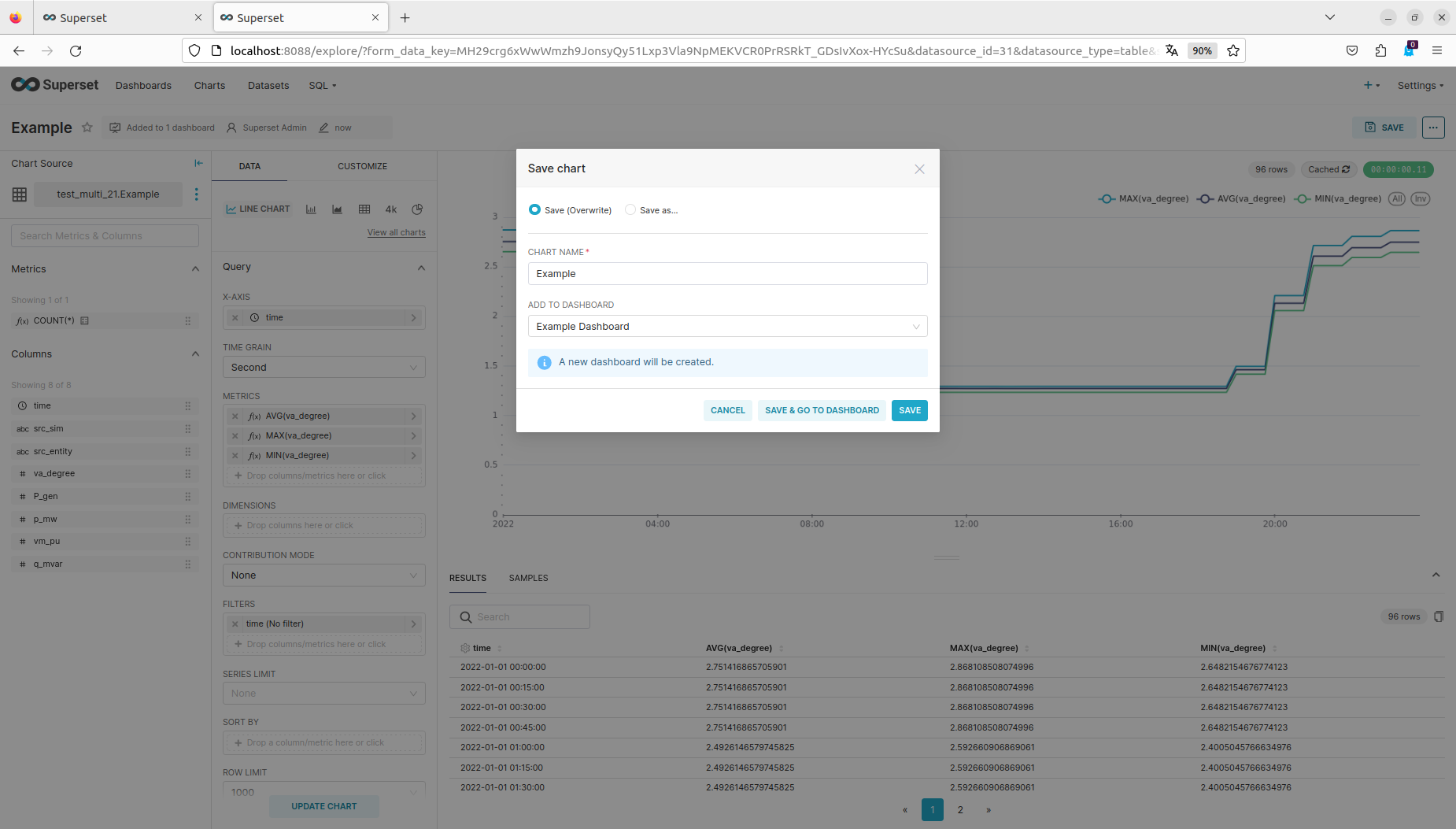
This is the saving menu of the chart view.
After saving the chart in a dashboard the created/picked dashboard can be found in the dashboard view.
This is the dashboard view.
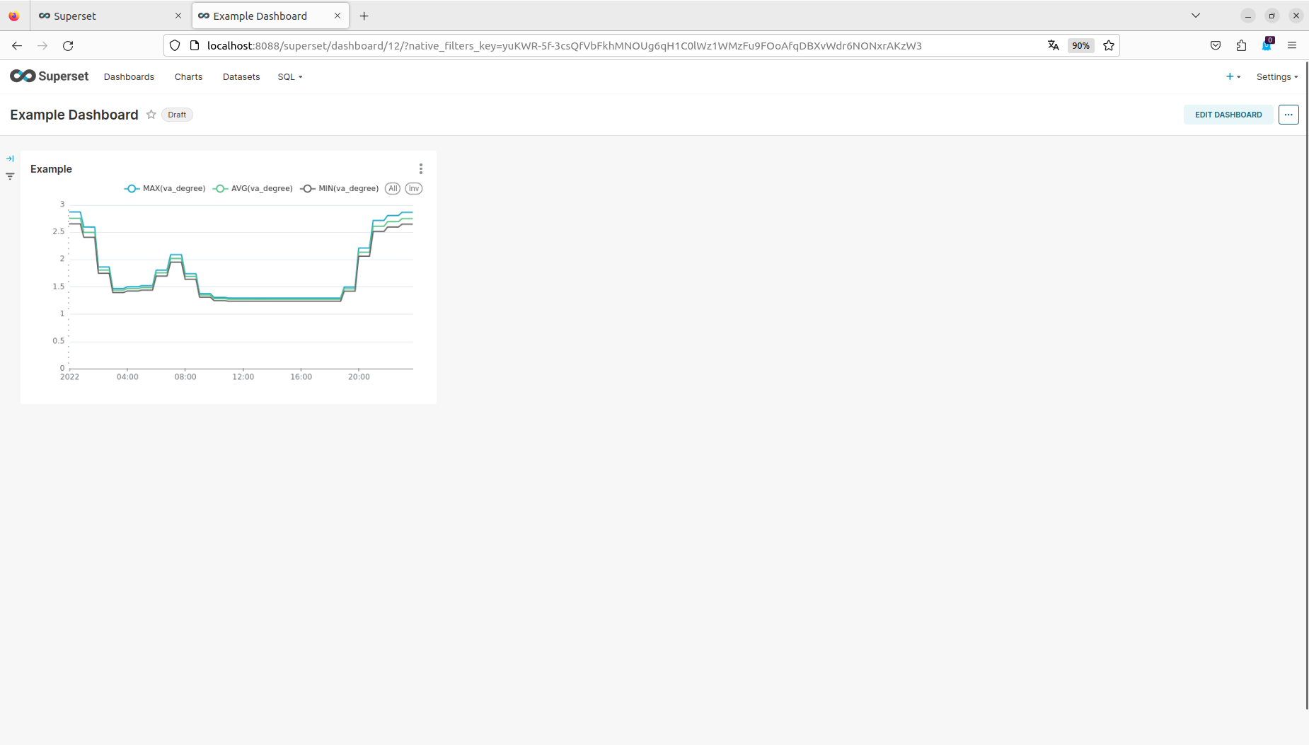
If a dashboard is selected it displays all charts that are saved in it.
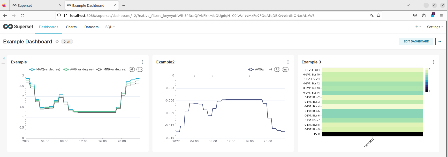
This is the created example dashboard.
Inside a dashboard charts can be updated, removed, looked at in fullscreen, exported and more.
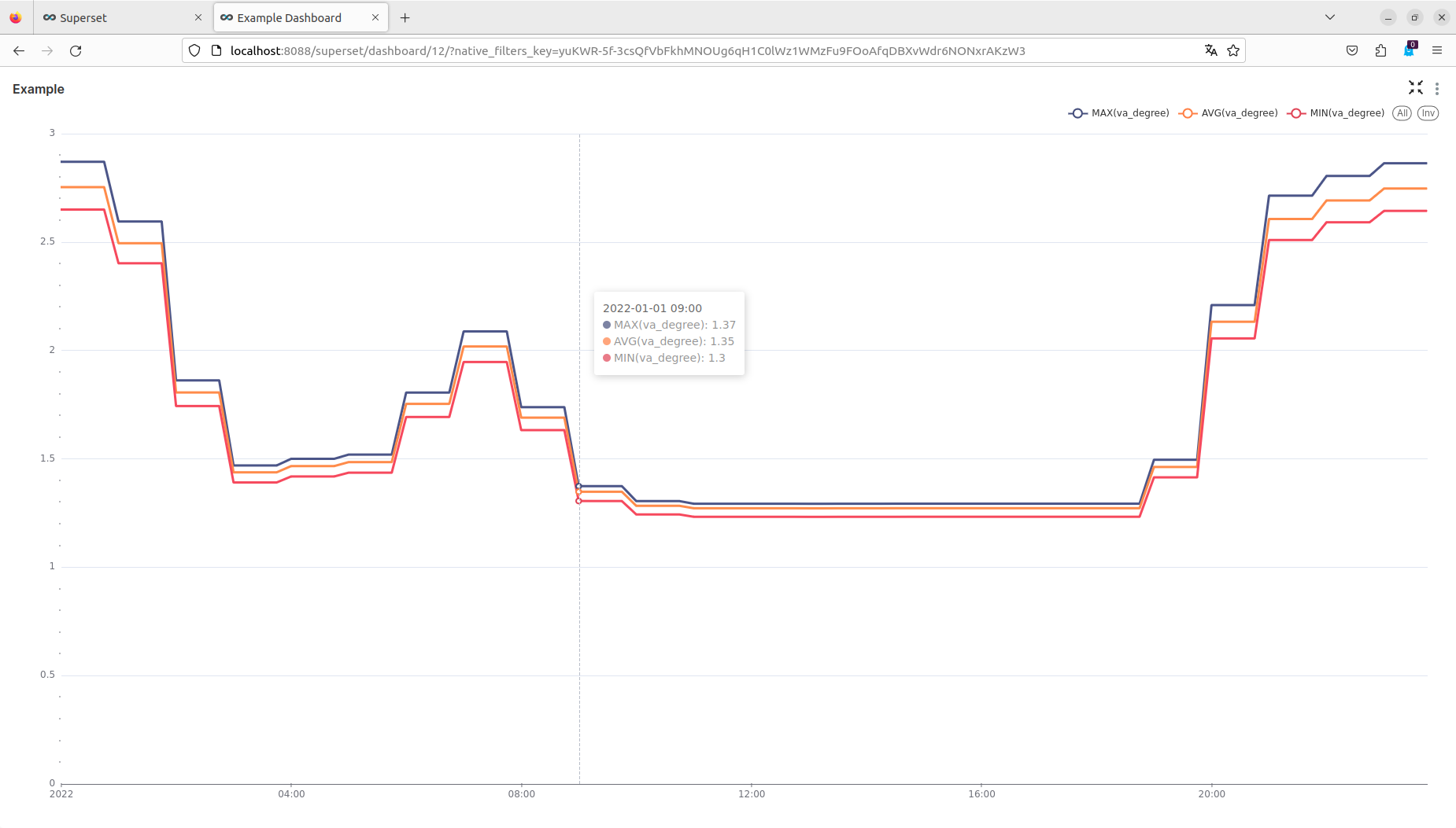
This is the created example chart in fullscreen.