Compressor efficiency map

The design case from the previous step can be used as the basis for offdesign calculations to predict the system’s performance (in terms of Electrical power/COP) at different operating conditions, i.e., a different source or consumer inlet temperature. While the tutorial in TESPy’s documentation provides a detailed explanation of all the changes between the two modes of calculations, only the most relevant changes are discussed here.

The refrigerant and the temperature difference for air in the evaporator remain unchanged. The source air temperature and the condenser inlet temperature are available as inputs to the model. The maximum heating capacity at a particular source air temperature is available from the datasheet. The condenser outlet temperature is not known in the off-design case, but must be predicted. In the design mode, the heating capacity and temperature difference between condenser inlet and outlet are used to calculate the mass flow in the circuit. This mass flow is used to calculate the condenser outlet temperature in the off-design mode.

In order to determine the electrical power consumption, the isentropic efficiency of the compressor is required. Since this is not available in the datasheets for the entire range of operation, the default characteristic curve available in the TESPy library, shown in figure below, is used.

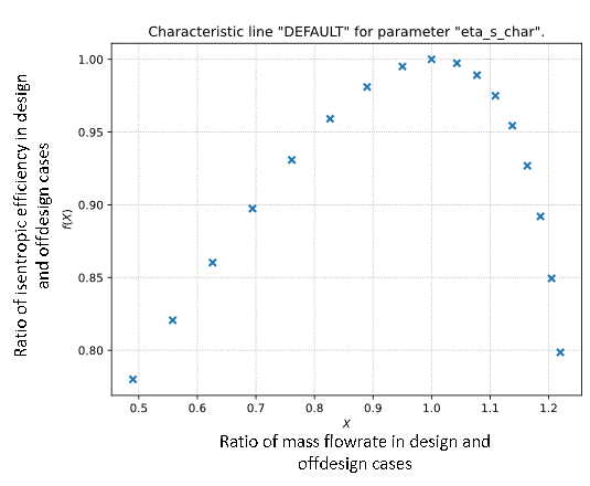
Default characteristic curve for the isentropic efficiency of the compressor in TESPy library

The x-axis is the ratio of the mass flow into the compressor in the design and off-design cases, and the y-axis is the ratio of the isentropic efficiencies in the design and off-design conditions.

The default characteristic curve is generic and therefore does not accurately reflect the performance of the specific model of the heat pump chosen. Instead of relying on the isentropic efficiency from a single design point and the default characteristic curve across the entire range of operation, a series of design points have been developed based on the data available in the manufacturer’s datasheet for the operating conditions shown in table 3.3.

Design point conditions
Source air temperatures (°C)	-20, -15, -12, -10, -7, -2, 2, 7, 10, 12, 15, 20, 25, 30, 35
Condenser outlet temperatures (°C)	15, 20, 25, 30, 35, 40, 45, 50, 55

The operating range of the heat pump for the source air temperature is -20°C to 35°C. The actual operation range of the heat pump on the condenser outlet temperature is 25°C to 60°C. In the model, the range is further increased to 15°C to 60°C, in order to simulate low temperature lift conditions. The temperature difference in the condenser, constant at 5°C in the design case, has been used to calculate the condenser inlet temperature.

Extension of the heating capacity table of the heat pump

The manufacturer’s datasheets contain the heating power curves and the electrical power curves as shown in figure below.

Heating capacity, electrical power, and COP curves of the chosen heat pump

In all the plots, the x-axis corresponds to the source (air) temperature. The data is available for the entire range of source air temperature, but only for two condenser outlet temperatures, 35°C and 55°C.

The heating capacity increases with an increase in the source air temperature, but does not change significantly with a change in the condenser outlet temperature. At a given source air temperature, the heating capacity for all the other condenser outlet temperatures is assumed to be the average of the heating capacities at 35°C and 55°C.

The power consumption changes with both the source air temperature and the condenser outlet temperature. An approach based on Carnot efficiency has been used to predict the power consumption at the condenser outlet temperatures other than 35°C and 55°C. The ideal COP is calculated for all the operating points, using the equation below (note that the temperatures have to be in Kelvin scale).

For the operating points where the power consumption/COP is known, the Carnot efficiency has been calculated using the following equation.

The temperature lift for all the operating points is calculated using equation below

A second order polynomial equation has been fit to the pairs of the Carnot efficiencies and the corresponding temperature lifts, of operating points with condenser outlet temperatures 35°C and 55°C, as shown in figure below.

Carnot efficiency/COP vs Temperature Lift plot for the chosen heat pump

In this figure, the COP of the heat pump is also plotted against the temperature lift. The Carnot efficiencies of the remaining operating points are estimated using the fit equation, which in turn are used to estimate the real COP/power consumption.

For the series of design points identified, the calculated heating capacity and power consumption data is summarized in the table below.

Expanded heating capacity table of the heat pump

The heating capacity data has to be saved in the ‘Heat_Load_Data.csv’ file and the power consumption data has to be saved in the ‘PI_Data.csv’ file.

Generating the compressor efficiency map

The tutorial available in the ‘script_etas_gen.ipynb’ is followed to generate the compressor efficiency map. The model is parametrized for each of the design point in the expanded heating capacity table from the previous step, as done for the initial parametrization of the model for the nominal operating point. As the power consumption of the compressor is dependent on the isentropic efficiency, which is set as a parameter in the compressor, it is changed for each point in order to match the power consumption calculated by the model and that in the table. The isentropic efficiency values are restricted to the range of 0.3 - 0.95.

Note

In the instances when the power values cannot be matched even at the extreme values for the compressor isentropic efficiency, the extreme values are assumed despite the difference in power predicted by the model and that in the table.

The compressor isentropic efficiency map generated as described is summarized in table below.